13.1	Banks will have flexibility in devising the precise nature of their expected shortfall (ES) models, but the following minimum standards will apply for the purpose of calculating market risk capital requirements. Banks subject to SAMA approval can apply stricter standards.
The IMA does not require all products to be simulated on full revaluation. Simplifications (eg sensitivities-based valuation) may be used provided SAMA agrees that the method used is adequate for the instruments covered.
13.2	ES must be computed on a daily basis for the bank-wide internal models to determine market risk capital requirements. ES must also be computed on a daily basis for each trading desk that uses the internal models approach (IMA).
13.3	In calculating ES, a bank must use a 97.5th percentile, one-tailed confidence level.
13.4	In calculating ES, the liquidity horizons described in [13.12] must be reflected by scaling an ES calculated on a base horizon. The ES for a liquidity horizon must be calculated from an ES at a base liquidity horizon of 10 days with scaling applied to this base horizon result as expressed below, where:
	(1)	ES is the regulatory liquidity-adjusted ES;
	(2)	T is the length of the base horizon, ie 10 days;
	(3)	EST(P) is the ES at horizon T of a portfolio with positions P = (pi) with respect to shocks to all risk factors that the positions P are exposed to;
	(4)	EST(P, j) is the ES at horizon T of a portfolio with positions P = (pi) with respect to shocks for each position pi in the subset of risk factors Q(pi, j), with all other risk factors held constant;
	(5)	the ES at horizon T, EST(P) must be calculated for changes in the risk factors, and EST(P, j) must be calculated for changes in the relevant subset Q(pi, j) of risk factors, over the time interval T without scaling from a shorter horizon;
	(6)	Q(pi, j)j is the subset of risk factors for which liquidity horizons, as specified in [13.12], for the desk where pi is booked are at least as long as LHj according to the table below. For example, Q(pi,4) is the set of risk factors with a 60-day horizon and a 120-day liquidity horizon. Note that Q(pi, j) is a subset of Q(pi, j–1);
	(7)	the time series of changes in risk factors over the base time interval T may be determined by overlapping observations; and
	(8)	LHj is the liquidity horizon j, with lengths in the following table:
Liquidity horizons, j Table 1 j LHj 1 10 2 20 3 40 4 60 5 120
13.5	The ES measure must be calibrated to a period of stress.
	(1)	Specifically, the ES measure must replicate an ES outcome that would be generated on the bank’s current portfolio if the relevant risk factors were experiencing a period of stress. This is a joint assessment across all relevant risk factors, which will capture stressed correlation measures.
	(2)	This calibration is to be based on an indirect approach using a reduced set of risk factors. Banks must specify a reduced set of risk factors that are relevant for their portfolio and for which there is a sufficiently long history of observations.
		(a)	This reduced set of risk factors is subject to SAMA approval and must meet the data quality requirements for a modellable risk factor as outlined in [11.12] to [11.24].
		(b)	The identified reduced set of risk factors must be able to explain a minimum of 75% of the variation of the full ES model (ie the ES of the reduced set of risk factors should be at least equal to 75% of the fully specified ES model on average measured over the preceding 12- week period).
The indicator that must be maximised for the identification of the stressed period is the aggregate capital requirement for modellable risk factors (IMCC) as per [13.15], it has to be maximised for the modellable risk factors, which implies that ESr,s is maximised, as noted in [13.7].
The reduced set of risk factors must be able to explain a minimum of 75% of the variation of the full ES model at the group level for the aggregate of all desks with IMA model approval.
13.6	The ES for market risk capital purposes is therefore expressed as follows, where:
	(1)	The ES for the portfolio using the above reduced set of risk factors (ESR,S), is calculated based on the most severe 12-month period of stress available over the observation horizon.
	(2)	ESR,S is then scaled up by the ratio of (i) the current ES using the full set of risk factors to (ii) the current ES measure using the reduced set of factors. For the purpose of this calculation, this ratio is floored at 1.
		(a)	ESF,C is the ES measure based on the current (most recent) 12-month observation period with the full set of risk factors; and
		(b)	ESR,C is the ES measure based on the current period with a reduced set of risk factors.
13.7	For measures based on stressed observations (ESR,S), banks must identify the 12-month period of stress over the observation horizon in which the portfolio experiences the largest loss. The observation horizon for determining the most stressful 12 months must, at a minimum, span back to and include 2007. Observations within this period must be equally weighted. Banks must update their 12- month stressed periods at least quarterly, or whenever there are material changes in the risk factors in the portfolio. Whenever a bank updates its 12-month stressed periods it must also update the reduced set of risk factors (as the basis for the calculations of ER,C and ER,S) accordingly.
13.8	For measures based on current observations (ESF,C), banks must update their data sets no less frequently than once every three months and must also reassess data sets whenever market prices are subject to material changes.
	(1)	This updating process must be flexible enough to allow for more frequent updates.
	(2)	SAMA may also require a bank to calculate its ES using a shorter observation period if, in SAMA’s judgement; this is justified by a significant upsurge in price volatility. In this case, however, the period should be no shorter than six months.
13.9	No particular type of ES model is prescribed. Provided that each model used captures all the material risks run by the bank, as confirmed through profit and loss (P&L) attribution (PLA) tests and backtesting, and conforms to each of the requirements set out above and below, SAMA may permit banks to use models based on either historical simulation, Monte Carlo simulation, or other appropriate analytical methods.
13.10	Banks will have discretion to recognise empirical correlations within broad regulatory risk factor classes (interest rate risk, equity risk, foreign exchange risk, commodity risk and credit risk, including related options volatilities in each risk factor category). Empirical correlations across broad risk factor categories will be constrained by SAMA aggregation requirements, as described in [13.14] to [13.15], and must be calculated and used in a manner consistent with the applicable liquidity horizons, clearly documented and able to be explained to SAMA on request.
13.11	Banks’ models must accurately capture the risks associated with options within each of the broad risk categories. The following criteria apply to the measurement of options risk:
	(1)	Banks’ models must capture the non-linear price characteristics of options positions.
	(2)	Banks’ risk measurement systems must have a set of risk factors that captures the volatilities of the rates and prices underlying option positions, ie vega risk. Banks with relatively large and/or complex options portfolios must have detailed specifications of the relevant volatilities. Banks must model the volatility surface across both strike price and vertex (ie tenor).
13.12	As set out in [13.4], a scaled ES must be calculated based on the liquidity horizon n defined below. n is calculated per the following conditions:
	(1)	Banks must map each risk factor on to one of the risk factor categories shown below using consistent and clearly documented procedures.
	(2)	The mapping of risk factors must be:
		(a)	set out in writing;
		(b)	validated by the bank’s risk management;
		(c)	made available to SAMA; and
		(d)	subject to internal audit.
	(3)	n is determined for each broad category of risk factor as set out in Table 2. However, on a desk-by-desk basis, n can be increased relative to the values in the table below (ie the liquidity horizon specified below can be treated as a floor). Where n is increased, the increased horizon must be 20, 40, 60 or 120 days and the rationale must be documented and be subject to SAMA approval. Furthermore, liquidity horizons should be capped at the maturity of the related instrument.
Liquidity horizon n by risk factor Table 2 Risk factor category n Risk factor category n Interest rate: specified currencies - EUR, USD, GBP, AUD, JPY, SEK, CAD and domestic currency of a bank 10 Equity price (small cap): volatility 60 Interest rate: unspecified currencies 20 Equity: other types 60 Interest rate: volatility 60 Foreign exchange (FX) rate: specified currency pairs49 10 Interest rate: other types 60 FX rate: currency pairs 20 Credit spread: sovereign (investment grade, or IG) 20 FX: volatility 40 Credit spread: sovereign (high yield, or HY) 40 FX: other types 40 Credit spread: corporate (IG) 40 Energy and carbon emissions trading price 20 Credit spread: corporate (HY) 60 Precious metals and non-ferrous metals price 20 Credit spread: volatility 120 Other commodities price 60 Credit spread: other types 120 Energy and carbon emissions trading price: volatility 60   Precious metals and non-ferrous metals price: volatility 60 Equity price (large cap) 10 Other commodities price: volatility 120 Equity price (small cap) 20 Commodity: other types 120 Equity price (large cap): volatility 20
The liquidity horizon for equity large cap repo and dividend risk factors is 20 days. All other equity repo and dividend risk factors are subject to a liquidity horizon of 60 days.
For mono-currency and cross-currency basis risk, the liquidity horizons of 10 days and 20 days for interest rate-specified currencies and unspecified currencies, respectively, applied
The liquidity horizon for inflation risk factors should be consistent with the liquidity horizons for interest rate risk factors for a given currency.
If the maturity of the instrument is shorter than the respective liquidity horizon of the risk factor as prescribed in [13.12], the next longer liquidity horizon length (out of the lengths of 10, 20, 40, 60 or 120 days as set out in the paragraph) compared with the maturity of the instrument itself must be used. For example, although the liquidity horizon for interest rate volatility is prescribed as 60 days, if an instrument matures in 30 days, a 40-day liquidity horizon would apply for the instrument’s interest rate volatility.
To determine the liquidity horizon of multi-sector credit and equity indices, the respective liquidity horizons of the underlying instruments must be used. A weighted average of liquidity horizons of the instruments contained in the index must be determined by multiplying the liquidity horizon of each individual instrument by its weight in the index (ie the weight used to construct the index) and summing across all instruments. The liquidity horizon of the index is the shortest liquidity horizon (out of 10, 20, 40, 60 and 120 days) that is equal to or longer than the weighted average liquidity horizon. For example, if the weighted average liquidity horizon is 12 days, the liquidity horizon of the index would be 20 days.

⁴⁹ SAR/USD USD/EUR, USD/JPY, USD/GBP, USD/AUD, USD/CAD, USD/CHF, USD/MXN, USD/CNY, USD/NZD, USD/RUB, USD/HKD, USD/SGD, USD/TRY, USD/KRW, USD/SEK, USD/ZAR, USD/INR, USD/NOK, USD/BRL, EUR/JPY, EUR/GBP, EUR/CHF and JPY/AUD. Currency pairs forming first-order crosses across these specified currency pairs are also subject to the same liquidity horizon.

13.16	Capital requirements for each non-modellable risk factor (NMRF) are to be determined using a stress scenario that is calibrated to be at least as prudent as the ES calibration used for modelled risks (ie a loss calibrated to a 97.5% confidence threshold over a period of stress). In determining that period of stress, a bank must determine a common 12-month period of stress across all NMRFs in the same risk class. Subject to SAMA approval, a bank may be permitted to calculate stress scenario capital requirements at the bucket level (using the same buckets that the bank uses to disprove modellability, per [11.16]) for risk factors that belong to curves, surfaces or cubes (ie a single stress scenario capital requirement for all the NMRFs that belong to the same bucket).
	(1)	For each NMRF, the liquidity horizon of the stress scenario must be the greater of the liquidity horizon assigned to the risk factor in [13.12] and 20 days. SAMA may require a higher liquidity horizon.
	(2)	For NMRFs arising from idiosyncratic credit spread risk, banks may apply a common 12- month stress period. Likewise, for NMRFs arising from idiosyncratic equity risk arising from spot, futures and forward prices, equity repo rates, dividends and volatilities, banks may apply a common 12-month stress scenario. Additionally, a zero correlation assumption may be used when aggregating gains and losses provided the bank conducts analysis to demonstrate to SAMA that this is appropriate.50 Correlation or diversification effects between other non-idiosyncratic NMRFs are recognised through the formula set out in [13.17].
	(3)	In the event that a bank cannot provide a stress scenario which is acceptable for SAMA, the bank will have to use the maximum possible loss as the stress scenario.
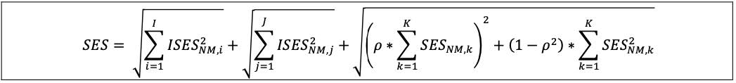
13.17	The aggregate regulatory capital measure for I (non-modellable idiosyncratic credit spread risk factors that have been demonstrated to be appropriate to aggregate with zero correlation), J (non-modellable idiosyncratic equity risk factors that have been demonstrated to be appropriate to aggregate with zero correlation) and the remaining K (risk factors in model-eligible trading desks that are non-modellable (SES)) is calculated as follows, where:
	(1)	ISESNM,i is the stress scenario capital requirement for idiosyncratic credit spread non- modellable risk i from the I risk factors aggregated with zero correlation;
	(2)	ISES NM,j is the stress scenario capital requirement for idiosyncratic equity non-modellable risk j from the J risk factors aggregated with zero correlation;
	(3)	SESNM,k is the stress scenario capital requirement for non-modellable risk k from K risk factors; and
	(4)	Rho (ρ) is equal to 0.6.

⁵⁰ The tests are generally done on the residuals of panel regressions where the dependent variable is the change in issuer spread while the independent variables can be either a change in a market factor or a dummy variable for sector and/or region. The assumption is that the data on the names used to estimate the model suitably proxies the names in the portfolio and the idiosyncratic residual component captures the multifactor-name basis. If the model is missing systematic explanatory factors or the data suffers from measurement error, then the residuals would exhibit heteroscedasticity (which can be tested via White, Breuche Pagan tests etc) and/or serial correlation (which can be tested with Durbin Watson, Lagrange multiplier (LM) tests etc) and/or cross-sectional correlation (clustering).

13.18	Banks must have a separate internal model to measure the default risk of trading book positions. The general criteria in [10.1] to [10.4] and the qualitative standards in [10.5] to [10.16] also apply to the default risk model.
13.19	Default risk is the risk of direct loss due to an obligor’s default as well as the potential for indirect losses that may arise from a default event.
13.20	Default risk must be measured using a value-at-risk (VaR) model.
	(1)	Banks must use a default simulation model with two types of systematic risk factors.
	(2)	Default correlations must be based on credit spreads or on listed equity prices. Correlations must be based on data covering a period of 10 years that includes a period of stress as defined in [13.5] and based on a one-year liquidity horizon.
	(3)	Banks must have clear policies and procedures that describe the correlation calibration process, documenting in particular in which cases credit spreads or equity prices are used.
	(4)	Banks have the discretion to apply a minimum liquidity horizon of 60 days to the determination of default risk capital (DRC) requirement for equity sub-portfolios.
	(5)	The VaR calculation must be conducted weekly and be based on a one-year time horizon at a one-tail, 99.9 percentile confidence level.
Banks are permitted to calibrate correlations to liquidity horizons of 60 days in the case that a separate calculation is performed for equity sub-portfolios and these desks deal predominately in equity exposures. In the case of a desk with both equity and bond exposures, for which a joint calculation for default risk of equities and bonds needs to be performed, the correlations need to be calibrated to a liquidity horizon of one year. In this case, a bank is permitted to consistently use a 60-day probability of default (PD) for equities and a one-year PD for bonds.
[13.20](2) states: “Default correlations must be based on credit spreads or on listed equity prices.” No additional data sources (eg rating time series) are permitted
[13.20](1) specifies that banks must use a default simulation model with two types of systematic risk factors. To meet this condition, the model always have two random variables that correspond to the systematic risk factors. Systematic risk in a DRC requirement model must be accounted for via multiple systematic factors of two different types. The rando variable that determines whether an obligor defaults must be an obligor-specific function of the systematic factors of both types and of an idiosyncratic factor. For example, in a Merton-type model, obligor i defaults when its asset return X falls below an obligor-specific threshold that determines the obligor’s probability of default. Systematic risk can be described via M systematic regional factors Yjreglon(j = 1, ... , M) and N systematic industry factors Yjindustry (j= 1, ... , N). For each obligor i, region factor loadings Bi,jregionand industry factor loadings Bi,jindustry that describe the sensitivity of the obligor’s asset return to each systematic factor need to be chosen. There must be at least one non-zero factor loading for the region type and at least one non-zero factor loading for the industry type. The asset return of obligor i can be represented as X? =ΣBi,jregion ∙ Yjregion +Σ Bi,jindustry ∙ Yjindustry+?? ∙??, where εi is the idiosyncratic risk factor and γi is the idiosyncratic factor loading.
Banks are permitted to use a 60-day liquidity horizon for all equity positions but are permitted to use a longer liquidity horizon where appropriate
13.21	All positions subject to market risk capital requirements that have default risk as defined in [13.19], with the exception of those positions subject to the standardised approach, are subject to the DRC requirement model.
	(1)	Sovereign exposures (including those denominated in the sovereign’s domestic currency), equity positions and defaulted debt positions must be included in the model.
	(2)	For equity positions, the default of an issuer must be modelled as resulting in the equity price dropping to zero.
13.22	The DRC requirement model capital requirement is the greater of:
	(1)	the average of the DRC requirement model measures over the previous 12 weeks; or
	(2)	the most recent DRC requirement model measure.
13.23	A bank must assume constant positions over the one-year horizon, or 60 days in the context of designated equity sub-portfolios.
The concept of constant positions has changed in the market risk framework because the capital horizon is now meant to always be synonymous with the new definition of liquidity horizon and no new positions are added when positions expire during the capital horizon. For securities with a maturity under one year, a constant position can be maintained within the liquidity horizon but, any maturity of a long or short position must be accounted for when the ability to maintain a constant position within the liquidity horizon cannot be contractually assured.
13.24	Default risk must be measured for each obligor.
	(1)	Probabilities of default (PDs) implied from market prices are not acceptable unless they are corrected to obtain an objective probability of default.51
	(2)	PDs are subject to a floor of 0.03%.
13.25	A bank’s model may reflect netting of long and short exposures to the same obligor. If such exposures span different instruments with exposure to the same obligor, the effect of the netting must account for different losses in the different instruments (eg differences in seniority).
13.26	The basis risk between long and short exposures of different obligors must be modelled explicitly. The potential for offsetting default risk among long and short exposures across different obligors must be included through the modelling of defaults. The pre-netting of positions before input into the model other than as described in [13.25] is not allowed.
13.27	The DRC requirement model must recognise the impact of correlations between defaults among obligors, including the effect on correlations of periods of stress as described below.
	(1)	These correlations must be based on objective data and not chosen in an opportunistic way where a higher correlation is used for portfolios with a mix of long and short positions and a low correlation used for portfolios with long only exposures.
	(2)	A bank must validate that its modelling approach for these correlations is appropriate for its portfolio, including the choice and weights of its systematic risk factors. A bank must document its modelling approach and the period of time used to calibrate the model.
	(3)	These correlations must be measured over a liquidity horizon of one year.
	(4)	These correlations must be calibrated over a period of at least 10 years.
	(5)	Banks must reflect all significant basis risks in recognising these correlations, including, for example, maturity mismatches, internal or external ratings, vintage etc.
13.28	The bank’s model must capture any material mismatch between a position and its hedge. With respect to default risk within the one-year capital horizon, the model must account for the risk in the timing of defaults to capture the relative risk from the maturity mismatch of long and short positions of less than one-year maturity.
13.29	The bank’s model must reflect the effect of issuer and market concentrations, as well as concentrations that can arise within and across product classes during stressed conditions.
13.30	As part of this DRC requirement model, the bank must calculate, for each and every position subjected to the model, an incremental loss amount relative to the current valuation that the bank would incur in the event that the obligor of the position defaults.
13.31	Loss estimates must reflect the economic cycle; for example, the model must incorporate the dependence of the recovery on the systemic risk factors.
13.32	The bank’s model must reflect the non-linear impact of options and other positions with material non-linear behaviour with respect to default. In the case of equity derivatives positions with multiple underlyings, simplified modelling approaches (for example modelling approaches that rely solely on individual jump-to-default sensitivities to estimate losses when multiple underlyings default) may be applied (subject to SAMA approval).
The simplified treatment applies only to equity derivatives.
13.33	Default risk must be assessed from the perspective of the incremental loss from default in excess of the mark-to-market losses already taken into account in the current valuation.
13.34	Owing to the high confidence standard and long capital horizon of the DRC requirement, robust direct validation of the DRC model through standard backtesting methods at the 99.9%/one-year soundness standard will not be possible.
	(1)	Accordingly, validation of a DRC model necessarily must rely more heavily on indirect methods including but not limited to stress tests, sensitivity analyses and scenario analyses, to assess its qualitative and quantitative reasonableness, particularly with regard to the model’s treatment of concentrations.
	(2)	Given the nature of the DRC soundness standard, such tests must not be limited to the range of events experienced historically.
	(3)	The validation of a DRC model represents an ongoing process in which supervisors and firms jointly determine the exact set of validation procedures to be employed.
13.35	Banks should strive to develop relevant internal modelling benchmarks to assess the overall accuracy of their DRC models.
13.36	Due to the unique relationship between credit spread and default risk, banks must seek SAMA approval for each trading desk with exposure to these risks, both for credit spread risk and default risk. Trading desks which do not receive SAMA approval will be deemed ineligible for internal modelling standards and be subject to the standardised capital framework.
13.37	Where a bank has approved PD estimates as part of the internal ratings-based (IRB) approach, this data must be used. Where such estimates do not exist, or SAMA determines that they are not sufficiently robust, PDs must be computed using a methodology consistent with the IRB methodology and satisfy the following conditions.
	(1)	Risk-neutral PDs should not be used as estimates of observed (historical) PDs.
	(2)	PDs must be measured based on historical default data including both formal default events and price declines equivalent to default losses. Where possible, this data should be based on publicly traded securities over a complete economic cycle. The minimum historical observation period for calibration purposes is five years.
	(3)	PDs must be estimated based on historical data of default frequency over a one-year period. The PD may also be calculated on a theoretical basis (eg geometric scaling) provided that the bank is able to demonstrate that such theoretical derivations are in line with historical default experience.
	(4)	PDs provided by external sources may also be used by banks, provided they can be shown to be relevant for the bank’s portfolio.
13.38	Where a bank has approved loss-given-default (LGD)52 estimates as part of the IRB approach, this data must be used. Where such estimates do not exist, or SAMA determines that they are not sufficiently robust, LGDs must be computed using a methodology consistent with the IRB methodology and satisfy the following conditions.
	(1)	LGDs must be determined from a market perspective, based on a position’s current market value less the position’s expected market value subsequent to default. The LGD should reflect the type and seniority of the position and cannot be less than zero.
	(2)	LGDs must be based on an amount of historical data that is sufficient to derive robust, accurate estimates.
	(3)	LGDs provided by external sources may also be used by institutions, provided they can be shown to be relevant for the bank’s portfolio.
13.39	Banks must establish a hierarchy ranking their preferred sources for PDs and LGDs, in order to avoid the cherry-picking of parameters.

⁵¹ Market-implied PDs are not acceptable.
⁵² LGD should be interpreted in this context as 1 – recovery rate.