13.16	Capital requirements for each non-modellable risk factor (NMRF) are to be determined using a stress scenario that is calibrated to be at least as prudent as the ES calibration used for modelled risks (ie a loss calibrated to a 97.5% confidence threshold over a period of stress). In determining that period of stress, a bank must determine a common 12-month period of stress across all NMRFs in the same risk class. Subject to SAMA approval, a bank may be permitted to calculate stress scenario capital requirements at the bucket level (using the same buckets that the bank uses to disprove modellability, per [11.16]) for risk factors that belong to curves, surfaces or cubes (ie a single stress scenario capital requirement for all the NMRFs that belong to the same bucket).
	(1)	For each NMRF, the liquidity horizon of the stress scenario must be the greater of the liquidity horizon assigned to the risk factor in [13.12] and 20 days. SAMA may require a higher liquidity horizon.
	(2)	For NMRFs arising from idiosyncratic credit spread risk, banks may apply a common 12- month stress period. Likewise, for NMRFs arising from idiosyncratic equity risk arising from spot, futures and forward prices, equity repo rates, dividends and volatilities, banks may apply a common 12-month stress scenario. Additionally, a zero correlation assumption may be used when aggregating gains and losses provided the bank conducts analysis to demonstrate to SAMA that this is appropriate.50 Correlation or diversification effects between other non-idiosyncratic NMRFs are recognised through the formula set out in [13.17].
	(3)	In the event that a bank cannot provide a stress scenario which is acceptable for SAMA, the bank will have to use the maximum possible loss as the stress scenario.
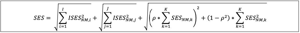
13.17	The aggregate regulatory capital measure for I (non-modellable idiosyncratic credit spread risk factors that have been demonstrated to be appropriate to aggregate with zero correlation), J (non-modellable idiosyncratic equity risk factors that have been demonstrated to be appropriate to aggregate with zero correlation) and the remaining K (risk factors in model-eligible trading desks that are non-modellable (SES)) is calculated as follows, where:
	(1)	ISESNM,i is the stress scenario capital requirement for idiosyncratic credit spread non- modellable risk i from the I risk factors aggregated with zero correlation;
	(2)	ISES NM,j is the stress scenario capital requirement for idiosyncratic equity non-modellable risk j from the J risk factors aggregated with zero correlation;
	(3)	SESNM,k is the stress scenario capital requirement for non-modellable risk k from K risk factors; and
	(4)	Rho (ρ) is equal to 0.6.

⁵⁰ The tests are generally done on the residuals of panel regressions where the dependent variable is the change in issuer spread while the independent variables can be either a change in a market factor or a dummy variable for sector and/or region. The assumption is that the data on the names used to estimate the model suitably proxies the names in the portfolio and the idiosyncratic residual component captures the multifactor-name basis. If the model is missing systematic explanatory factors or the data suffers from measurement error, then the residuals would exhibit heteroscedasticity (which can be tested via White, Breuche Pagan tests etc) and/or serial correlation (which can be tested with Durbin Watson, Lagrange multiplier (LM) tests etc) and/or cross-sectional correlation (clustering).