| 12.1. | This section sets out the calculation of exposure at default (EAD) for five sample portfolios using SA-CCR. The calculations for the sample portfolios assume that intermediate values are not rounded (i.e. the actual results are carried through in sequential order). However, for ease of presentation, these intermediate values as well as the final EAD are rounded.
|
| 12.2. | The EAD for all netting sets in SA-CCR is given by the following formula, where alpha is assigned a value of 1.4:
|
EAD = alpha * (RC + multiplier * AddOnaggregate
|
| | Example 1: Interest rate derivatives (unmargined netting set)
|
| 12.3. | Netting set 1 consists of three interest rates derivatives: two fixed versus floating interest rate swaps and one purchased physically-settled European swaption. The table below summarizes the relevant contractual terms of the three derivatives. All notional amounts and market values in the table are given in USD thousands.
|
| Trade # | Nature | Residual maturity | Base currency | Notional (USD thousands) | Pay Leg (*) | Receive Leg (*) | Market value (USD thousands) | | 1 | Interest Rate Swap | 10 years | USD | 10,000 | Fixed | Floating | 30 | | 2 | Interest Rate Swap | 4 years | USD | 10,000 | Floating | Fixed | -20 | | 3 | European Swaption | 1 into 10 years | EUR | 5,000 | Floating | Fixed | 50 | | (*) For the swaption, the legs are those of the underlying swap |
|
| 12.4. | The netting set is not subject to a margin agreement and there is no exchange of collateral (independent amount/initial margin) at inception. For unmargined netting sets, the replacement cost is calculated using the following formula, where:
|
| | (1) | V is a simple algebraic sum of the derivatives' market values at the reference date
|
| | (2) | C is the haircut value of the initial margin, which is zero in this example
|
RC = max{V - C; 0}
|
| 12.5. | Thus, using the market values indicated in the table (expressed in USD thousands):
|
RC = max{30 — 20 + 50 — 0; 0} = 60
|
| 12.6. | Since V-C is positive (i.e. USD 60,000), the value of the multiplier is 1, as explained in 6.24.
|
| 12.7. | The remaining term to be calculated in the calculation EAD is the aggregate add-on (AddOnaggregate). All the transactions in the netting set belong to the interest rate asset class. The AddOnaggregate for the interest rate asset class can be calculated using the seven steps set out in 6.60.
|
| 12.8. | Step 1: Calculate the effective notional for each trade in the netting set. This is calculated as the product of the following three terms:
|
| | (i) | the adjusted notional of the trade (d);
|
| | (ii) | the supervisory delta adjustment of the trade (δ); and
|
| | (iii) | the maturity factor (MF). That is, for each trade i, the effective notional Di is calculated as Di = di * MFi * δ.
|
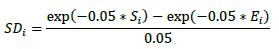
| 12.9. | For interest rate derivatives, the trade-level adjusted notional (di) is the product of the trade notional amount and the supervisory duration (SDi), i.e. di = notional * SDi. The supervisory duration is calculated using the following formula, where:
|
| | (1) | Si and Ei are the start and end dates, respectively, of the time period referenced by the interest rate derivative (or, where such a derivative references the value of another interest rate instrument, the time period determined on the basis of the underlying instrument). If the start date has occurred (e.g. an ongoing interest rate swap), Si must be set to zero.
|
| | (2) | The calculated value of SDi is floored at 10 business days (which expressed in years, using an assumed market convention of 250 business days a year is 10/250 years
|
| | |  |
| 12.10. | Using the formula for supervisory duration above, the trade-level adjusted notional amounts for each of the trades in Example 1 are as follows:
|
| | | Trade # | Notional (USD thousand) | Si | Ei | SDi | Adjusted notional, di (USD thousands) | | 1 | 10,000 | 0 | 10 | 7.87 | 78,694 | | 2 | 10,000 | 0 | 4 | 3.63 | 36,254 | | 3 | 5,000 | 1 | 11 | 7.49 | 37,428 |
|
| 12.11. | 6.51 sets out the calculation of the maturity factor (MFi) for unmargined trades. For trades that have a remaining maturity in excess of one year, which is the case for all trades in this example, the formula gives a maturity factor of 1.
|
| 12.12. | As set out in 6.40 to 6.43, a supervisory delta is assigned to each trade. In particular:
|
| | (1) | Trade 1 is long in the primary risk factor (the reference floating rate) and is not an option so the supervisory delta is equal to 1.
|
| | (2) | Trade 2 is short in the primary risk factor and is not an option; thus, the supervisory delta is equal to -1.
|
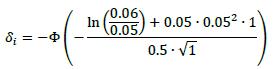
| | (3) | Trade 3 is an option to enter into an interest rate swap that is short in the primary risk factor and therefore is treated as a bought put option. As such, the supervisory delta is determined by applying the relevant formula in 6.42, using 50% as the supervisory option volatility and 1 (year) as the option exercise date. In particular, assuming that the underlying price (the appropriate forward swap rate) is 6% and the strike price (the swaption's fixed rate) is 5%, the supervisory delta is:
|
| | |  |
| 12.13. | The effective notional for each trade in the netting set (Di) is calculated using the formula Di = di * MFi * δi and values for each term noted above. The results of applying the formula are as follows:
|
| Trade # | Notional (USD thousands) | Adjusted notional, di (USD, thousands) | Maturity Factor, MFi | Delta, δi | Effective notional, Di (USD, thousands) | | 1 | 10,000 | 78,694 | 1 | 1 | 78,694 | | 2 | 10,000 | 36,254 | 1 | -1 | -36,254 | | 3 | 5,000 | 37,428 | 1 | -0.2694 | -10,083 |
|
| 12.14. | Step 2: Allocate the trades to hedging sets. In the interest rate asset class the hedging sets consist of all the derivatives that reference the same currency. In this example, the netting set is comprised of two hedging sets, since the trades refer to interest rates denominated in two different currencies (USD and EUR).
|
| 12.15. | Step 3: Within each hedging set allocate each of the trades to the following three maturity buckets: less than one year (bucket 1), between one and five years (bucket 2) and more than five years (bucket 3). For this example, within the hedging set “USD”, trade 1 falls into the third maturity bucket (more than 5 years) and trade 2 falls into the second maturity bucket (between one and five years). Trade 3 falls into the third maturity bucket (more than 5 years) of the hedging set “EUR”. The results of steps 1 to 3 are summarized in the table below:
|
| | | Trade # | Effective notional, Di (USD, thousands) | Hedging set | Maturity bucket | | 1 | 78,694 | USD | 3 | | 2 | -36,254 | USD | 2 | | 3 | -10,083 | EUR | 3 |
|
| 12.16. | Step 4: Calculate the effective notional of each maturity bucket (DB1, DB2 and DB3) within each hedging set (USD and EUR) by adding together all the trade level effective notionals within each maturity bucket in the hedging set. In this example, there are no maturity buckets within a hedging set with more than one trade, and so this case the effective notional of each maturity bucket is simply equal to the effective notional of the single trade in each bucket. Specifically:
|
| | (1) | For the USD hedging set: DB1 is zero, DB2 is -36,254 (thousand USD) and DB3 is 78,694 (thousand USD)
|
| | (2) | For the EUR hedging set: DB1 and DB2 are zero and DB3 is -10,083 (thousand USD).
|
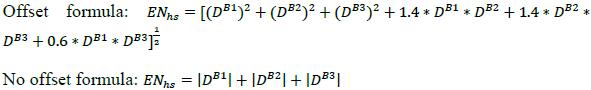
| 12.17. | Step 5: Calculate the effective notional of the hedging set (ENHS) by using either of the two following aggregation formulas (the latter is to be used if the bank chooses not to recognize offsets between long and short positions across maturity buckets):
|
| |  |
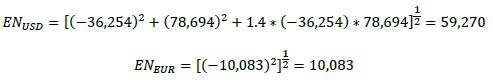
| 12.18. | In this example, the first of the two aggregation formulas is used. Therefore, the effective notionals for the USD hedging set (ENUSD) and the EUR hedging (ENEUR) are, respectively (expressed in USD thousands):
|
| |  |
| 12.19. | Step 6: Calculate the hedging set level add-on (AddOnhs) by multiplying the effective notional of the hedging set (ENhs) by the prescribed supervisory factor (SFhs). The prescribed supervisory factor in the interest rate asset class is set at 0.5%. Therefore, the add-on for the USD and EUR hedging sets are, respectively (expressed in USD thousands):
|
AddOnUSD = 59,270 ∗ 0.005 = 296.35
|
AddOnEUR = 10,083 ∗ 0.005 = 50.415
|
| 12.20. | Step 7: Calculate the asset class level add-on (AddOnIR) by adding together all of the hedging set level add-ons calculated in step 6. Therefore, the add-on for the interest rate asset class is (expressed in USD thousands):
|
AddOnIR = 296.35 + 50.415 = 347
|
| 12.21. | For this netting set the interest rate add-on is also the aggregate add-on because there are no derivatives belonging to other asset classes. The EAD for the netting set can now be calculated using the formula set out in 12.2 (expressed in USD thousands):
|
| | EAD = alpha * (RC + multip; ier * AddOnaggregate) = 1.4 * (60 + 1 * 347) = 569
|
| | Example 2: Credit derivatives (unmargined netting set)
|
| 12.22. | Netting set 2 consists of three credit derivatives: one long single-name credit default swap (CDS) written on Firm A (rated AA), one short single-name CDS written on Firm B (rated BBB), and one long CDS index (investment grade). The table below summarizes the relevant contractual terms of the three derivatives. All notional amounts and market values in the table are in USD thousands.
|
| Trade # | Nature | Reference entity/index name | Rating reference entity | Residual maturity | Base currency | Notional (USD thousands) | Position | Market value (USD thousands) | | 1 | Single name CDS | Firm A | AA | 3 years | USD | 10,000 | Protection buyer | 20 | | 2 | Single-name CDS | Firm B | BBB | 6 years | EUR | 10,000 | Protection seller | -40 | | 3 | CDS | CDX.IG 5y | Investment grade | 5 years | USD | 10,000 | Protection buyer | 0 |
|
| 12.23. | As in the previous example, the netting set is not subject to a margin agreement and there is no exchange of collateral (independent amount/IM) at inception. For unmargined netting sets, the replacement cost is calculated using the following formula, where:
|
| | (1) | V is a simple algebraic sum of the derivatives' market values at the reference date
|
| | (2) | C is the haircut value of the IM, which is zero in this example
|
RC = max{V - C; 0}
|
| 12.24. | Thus, using the market values indicated in the table (expressed in USD thousands):
|
RC = max{20 - 40 + 0 - 0; 0} = 0
|
| 12.25. | Since in this example V-C is negative (equal to V, i.e. -20,000), the multiplier will be activated (i.e. it will be less than 1). Before calculating its value, the aggregate add-on (AddOnaggregate) needs to be determined.
|
| 12.26. | All the transactions in the netting set belong to the credit derivatives asset class. The AddOnaggregate for the credit derivatives asset class can be calculated using the four steps set out in 6.64.
|
| 12.27. | Step 1: Calculate the effective notional for each trade in the netting set. This is calculated as the product of the following three terms: (i) the adjusted notional of the trade (d); (ii) the supervisory delta adjustment of the trade (δ); and (iii) the maturity factor (MF). That is, for each trade i, the effective notional Di is calculated as Di = di * MFi * δi.
|
| 12.28. | For credit derivatives, like interest rate derivatives, the trade-level adjusted notional (di) is the product of the trade notional amount and the supervisory duration (SDi), i.e. di = notional * SDi. The trade-level adjusted notional amounts for each of the trades in Example 2 are as follows:
|
| | | Trade # | Notional (USD thousand) | Si | Ei | SDi | Adjusted notional, di (USD thousands) | | 1 | 10,000 | 0 | 3 | 2.79 | 27,858 | | 2 | 10,000 | 0 | 6 | 5.18 | 51,836 | | 3 | 5,000 | 0 | 5 | 4.42 | 44,240 |
|
| 12.29. | 6.51 sets out the calculation of the maturity factor (MFi) for unmargined trades. For trades that have a remaining maturity in excess of one year, which is the case for all trades in this example, the formula gives a maturity factor of 1.
|
| 12.30. | As set out in 6.40 to 6.43, a supervisory delta is assigned to each trade. In particular:
|
| | (1) | Trade 1 and Trade 3 are long in the primary risk factors (CDS spread) and are not options so the supervisory delta is equal to 1 for each trade.
|
| | (2) | Trade 2 is short in the primary risk factor and is not an option; thus, the supervisory delta is equal to -1.
|
| 12.31. | The effective notional for each trade in the netting set (Di) is calculated using the formula Di = di * MFi * δi and values for each term noted above. The results of applying the formula are as follows:
|
| Trade # | Notional (USD thousands) | Adjusted notional, di (USD, thousands) | Maturity Factor,MFi | Delta, δi | Effective notional, Di (USD, thousands) | | 1 | 10,000 | 27,858 | 1 | 1 | 27,858 | | 2 | 10,000 | 51,836 | 1 | -1 | -51,836 | | 3 | 10,000 | 44,240 | 1 | 1 | 44,240 |
|
| 12.32. | Step 2: Calculate the combined effective notional for all derivatives that reference the same entity. The combined effective notional of the entity (ENentity) is calculated by adding together the trade level effective notionals calculated in step 1 that reference that entity. However, since all the derivatives refer to different entities (single names/indices), the effective notional of the entity is simply equal to the trade level effective notional (Di) for each trade.
|
| 12.33. | Step 3: Calculate the add-on for each entity (AddOnentity) by multiplying the entity level effective notional in step 2 by the supervisory factor that is specified for that entity (SFentity). The supervisory factors are set out in table 2 in 6.75. A supervisory factor is assigned to each single-name entity based on the rating of the reference entity (0.38% for AA-rated firms and 0.54% for BBB-rated firms). For CDS indices, the SF is assigned according to whether the index is investment or speculative grade; in this example, its value is 0.38% since the index is investment grade. Thus, the entity level add-ons are the following (USD thousands):
|
| | | Reference Entity | Effective notional, Di (USD, thousands) | Supervisory factor, SFentity | Entity-level add-on, AddOnentity (= Di ∗ SFentity) | | Firm A | 27,858 | 0.38% | 106 | | Firm B | -51,836 | 0.54% | -280 | | CDX.IG | 44,240 | 0.38% | 168 |
|
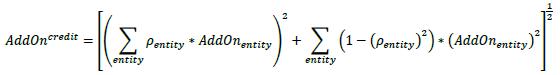
| 12.34. | Step 4: Calculate the asset class level add-on (AddOncredit) by using the formula that follows, where:
|
| | (1) | The summations are across all entities referenced by the derivatives.
|
| | (2) | AddOnentity is the add-on amount calculated in step 3 for each entity referenced by the derivatives.
|
| | (3) | ρentity is the supervisory prescribed correlation factor corresponding to the entity. As set out in Table 2 in 6.75, the correlation factor is 50% for single entities (Firm A and Firm B) and 80% for indexes (CDX.IG).
|
| |  |
| 12.35. | The following table shows a simple way to calculate of the systematic and idiosyncratic components in the formula:
|
| Reference Entity | Pentity | AddOnentity | Pentity∗ AddOnentity | 1 − (Pentity)2 | (AddOnentity )2 | (1 − (Pentity )2 ∗ (AddOnentity )2 | | Firm A | 0.5 | 106 | 52.9 | 0.75 | 11,207 | 8,405 | | Firm B | 0.5 | -280 | -140 | 0.75 | 78,353 | 58,765 | | CDX.IG | 0.8 | 168 | 134.5 | 0.36 | 28,261 | 101,174 | | Sum= | | | 47.5 | | | 77,344 | | (Sum)2= | | | 2,253 | | | |
|
| 12.36. | According to the calculations in the table, the systematic component is 2,253, while the idiosyncratic component is 77,344. Thus, the add-on for the credit asset class is calculated as follows:
|
| | 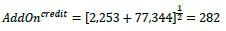 |
| 12.37. | For this netting set the credit add-on (AddOncredit) is also the aggregate add-on (AddOnaggregate) because there are no derivatives belonging to other asset classes.
|
| 12.38. | The value of the multiplier can now be calculated as follows, using the formula set out in 6.25:
|
| | 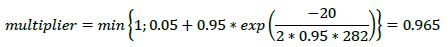 |
| 12.39. | Finally, aggregating the replacement cost and the potential future exposure (PFE) component and multiplying the result by the alpha factor of 1.4, the EAD is as follows (USD thousands):
|
| | EAD = 1.4 ∗ (0 + 0.965 ∗ 282) = 381
|
| | Example 3: Commodity derivatives (unmargined netting set)
|
| 12.40. | Netting set 3 consists of three commodity forward contracts. The table below summarizes the relevant contractual terms of the three derivatives. All notional amounts and market values in the table are in USD thousands.
|
| Trade # | Notional | Nature | Underlying | Direction | Residual maturity | Market value | | 1 | 10,000 | Forward | (West Texas Intermediate, or WTI) Crude Oil | Long | 9 months | -50 | | 2 | 20,000 | Forward | (Brent) Crude Oil | Short | 2 years | -30 | | 3 | 10,000 | Forward | Silver | Long | 5 years | -100 |
|
| 12.41. | As in the previous two examples, the netting set is not subject to a margin agreement and there is no exchange of collateral (independent amount/IM) at inception. Thus, the replacement cost is given by:
|
RC = max{V — C; 0} = max{100 — 30 — 50 — 0; 0} = 20
|
| 12.42. | Since V-C is positive (i.e. USD 20,000), the value of the multiplier is 1, as explained in 6.24.
|
| 12.43. | All the transactions in the netting set belong to the commodities derivatives asset class. The AddOnaggregate for the commodities derivatives asset class can be calculated using the six steps set out in 6.72.
|
| 12.44. | Step 1: Calculate the effective notional for each trade in the netting set. This is calculated as the product of the following three terms: (i) the adjusted notional of the trade (d); (ii) the supervisory delta adjustment of the trade (S); and (iii) the maturity factor (MF). That is, for each trade i, the effective notional DiD is calculated as Di = di * MFi * δi
|
| 12.45. | For commodity derivatives, the adjusted notional is defined as the product of the current price of one unit of the commodity (e.g. barrel of oil) and the number of units referenced by the derivative. In this example, for the sake of simplicity, it is assumed that the adjusted notional (di) is equal to the notional value.
|
| 12.46. | 6.51 sets out the calculation of the maturity factor (MFi) for unmargined trades. For trades that have a remaining maturity in excess of one year (trades 2 and 3 in this example), the formula gives a maturity factor of 1. For trade 1 the formula gives the following maturity factor:
|
| |  |
| 12.47. | As set out in 6.40 to 6.43, a supervisory delta is assigned to each trade. In particular:
|
| | (1) | Trade 1 and Trade 3 are long in the primary risk factors (WTI Crude Oil and Silver respectively) and are not options so the supervisory delta is equal to 1 for each trade.
|
| | (2) | Trade 2 is short in the primary risk factor (Brent Crude Oil) and is not an option; thus, the supervisory delta is equal to -1.
|
| Trade # | Notional (USD thousands) | Adjusted notional, di (USD, thousands) | Maturity Factor, MFi | Delta, δi | Effective notional, Di (USD, thousands) | | 1 | 10,000 | 10,000 | (9/12)0.5 | 1 | 8,660 | | 2 | 20,000 | 20,000 | 1 | -1 | -20,000 | | 3 | 10,000 | 10,000 | 1 | 1 | 10,000 |
|
| 12.48. | Step 2: Allocate the trades in commodities asset class to hedging sets. In the commodities asset class there are four hedging sets consisting of derivatives that reference: energy (trades 1 and 2 in this example), metals (trade 3 in this example), agriculture and other commodities.
|
| | | Hedging set | Commodity type | Trades | | Energy | Crude oil | 1 and 2 | | Natural gas | None | | Coal | None | | Electricity | None | | Metals | Silver | 3 | | Gold | None | | | ... | ... | | Agriculture | ... | ... | | ... | ... | | Other | ... | ... |
|
| | | Trade # | Effective notional, Di (USD thousands) | Hedging set | Commodity type | | 1 | 8,660 | Energy | Crude oil | | 2 | -20,000 | Energy | Crude Oil | | 3 | 10,000 | Metal | Silver |
|
| 12.49. | Step 3: Calculate the combined effective notional for all derivatives with each hedging set that reference the same commodity type. The combined effective notional of the commodity type (ENcomType) is calculated by adding together the trade level effective notionals calculated in step 1 that reference that commodity type. For purposes of this calculation, the bank can ignore the basis difference between the WTI and Brent forward contracts since they belong to the same commodity type, “Crude Oil” (unless the national supervisor requires the bank to use a more refined definition of commodity types). This step gives the following:
|
| | (1) | ENCrudeOil = 8,660 + (—20,000) = —11,340
|
| | (2) | ENSilver = 10,000
|
| 12.50. | Step 4: Calculate the add-on for each commodity type (AddOncomType) within each hedging set by multiplying the combined effective notional for that commodity calculated in step 3 by the supervisory factor that is specified for that commodity type (SFcomType). The supervisory factors are set out in table 2 in 6.75 and are set at 40% for electricity derivatives and 18% for derivatives that reference all other types of commodities. Therefore:
|
| | (1) | AddOnCrudeOil = -11,340 * 0.18 = -2,041
|
| | (2) | AddOnSilver = 10,000 * 0.18 = 1,800
|
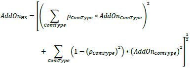
| 12.51. | Step 5: Calculate the add-on for each of the four commodity hedging sets (AddOnHS) by using the formula that follows. In the formula:
|
| | (1) | The summations are across all commodity types within the hedging set.
|
| | (2) | AddOnComType is the add-on amount calculated in step 4 for each commodity type.
|
| | (3) | ρComType is the supervisory prescribed correlation factor corresponding to the commodity type. As set out in Table 2 in 6.75, the correlation factor is set at 40% for all commodity types.
|
| | |  |
| 12.52. | In this example, however, there is only one commodity type within the “Energy” hedging set (ie Crude Oil). All other commodity types within the energy hedging set (eg coal, natural gas etc) have a zero add-on. Therefore, the add-on for the energy hedging set is calculated as follows:
|
| | 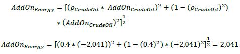 |
| 12.53. | The calculation above shows that, when there is only one commodity type within a hedging set, the hedging-set add-on is equal (in absolute value) to the commodity-type add-on.
|
| 12.54. | Similarly, “Silver” is the only commodity type in the “Metals” hedging set, and so the add-on for the metals hedging set is:
|
AddOnMetals = |AddOnSilver| = 1,800
|
| 12.55. | Step 6: Calculate the asset class level add-on (AddOnCommodity) by adding together all of the hedging set level add-ons calculated in step 5:
|
| | 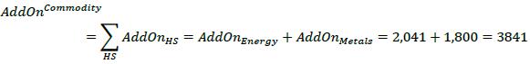 |
| 12.56. | For this netting set the commodity add-on (AddOnCommodity) is also the aggregate add-on (AddOnaggregate) because there are no derivatives belonging to other asset classes.
|
| 12.57. | Finally, aggregating the replacement cost and the PFE component and multiplying the result by the alpha factor of 1.4, the EAD is as follows (USD thousands):
|
EAD = 1.4 * (20 + 1 ∗ 3,841) = 5,406
|
| | Example 4: Interest rate and credit derivatives (unmargined netting set)
|
| 12.58. | Netting set 4 consists of the combined trades of Examples 1 and 2. There is no margin agreement and no collateral. The replacement cost of the combined netting set is:
|
RC = max{V - C;0} = max{30 − 20 + 50 + 20 − 40 + 0; 0} = 40
|
| 12.59. | The aggregate add-on for the combined netting set is the sum of add-ons for each asset class. In this case, there are two asset classes, interest rates and credit, and the add-ons for these asset classes have been copied from Examples 1 and 2:
|
AddOnaggregate = AddOnIR + AddOncredit = 347 + 282 = 629
|
| 12.60. | Because V-C is positive, the multiplier is equal to 1. Finally, the EAD can be calculated as:
|
EAD = 1.4 * (40 + 1 * 629) = 936
|
| | Example 5: Interest rate and commodities derivatives (unmargined netting set)
|
| 12.61. | Netting set 5 consists of the combined trades of Examples 1 and 3. However, instead of being unmargined (as assumed in those examples), the trades are subject to a margin agreement with the following specifications:
|
| Margin frequency | Threshold, TH | Minimum Transfer Amount, MTA | Independent Amount, IA | Total net collateral held by bank | | | | (USD thousands) | (USD thousands) | (USD thousands) | | Weekly | 0 | 5 | 150 | 200 |
|
| 12.62. | The above table depicts a situation in which the bank received from the counterparty a net independent amount of 150 (taking into account the net amount of initial margin posted by the counterparty and any unsegregated initial margin posted by the bank). The total net collateral (after the application of haircuts) currently held by the bank is 200, which includes 50 for variation margin (VM) received and 150 for the net independent amount.
|
| 12.63. | First, we determine the replacement cost. The net collateral currently held is 200 and the net independent collateral amount (NICA) is equal to the independent amount (that is, 150). The current market value of the trades in the netting set (V) is 80, it is calculated as the sum of the market value of the trades, i.e. 30 - 20 + 50 - 50 - 30 + 100 = 80. The replacement cost for margined netting sets is calculated using the formula set out in 6.20. Using this formula the replacement cost for the netting set in this example is:
|
RC = max{V — C; TH +MTA — NICA; 0} = max{80 — 200; 0 + 5 — 150; 0} = 0
|
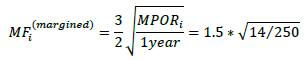
| 12.64. | Second, it is necessary to recalculate the interest rate and commodity add-ons, based on the value of the maturity factor for margined transactions, which depends on the margin period of risk. For daily re-margining, the margin period of risk (MPOR) would be 10 days. In accordance with 6.53, for netting sets that are not subject daily margin agreements the MPOR is the sum of nine business days plus the re-margining period (which is five business days in this example). Thus the MPOR is 14 (= 9 + 5) in this example.
|
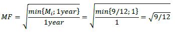
| 12.65. | The re-scaled maturity factor for the trades in the netting set is calculated using the formula set out in 6.55. Using the MPOR calculated above, the maturity factor for all trades in the netting set in this example it is calculated as follows (a market convention of 250 business days in the financial year is used):
|
| |  |
| 12.66. | For the interest rate add-on, the effective notional for each trade (Di = di ∗ MFi ∗ Ꟙi) calculated in 12.13 must be recalculated using the maturity factor for the margined netting set calculated above. That is:
|
| IR Trade # | Notional (USD thousands) | Base currency (hedging set) | Maturity bucket | Adjusted notional, di (USD, thousands) | Maturity Factor, MFi | Delta, Ꟙi | Effective notional, Di (USD, thousands) | | 1 | 10,000 | USD | 3 | 78,694 | 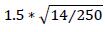 | 1 | 27,934 | | 2 | 10,000 | USD | 2 | 36,254 | | -1 | -12,869 | | 3 | 5,000 | EUR | 3 | 37,428 | | -0.2694 | -3,579 |
|
| 12.67. | Next, the effective notional of each of the three maturity buckets within each hedging set must now be calculated. However, as set out in 12.16, given that in this example there are no maturity buckets within a hedging set with more than a single trade, the effective maturity of each maturity bucket is simply equal to the effective notional of the single trade in each bucket. Specifically:
|
| | (1) | For the USD hedging set: DB1 is zero, DB2 is -12,869 (thousand USD) and DB3 is 27,934 (thousand USD).
|
| | (2) | For the EUR hedging set: DB1 and DB2 are zero and DB3 is -3,579 (thousand USD).
|
| 12.68. | Next, the effective notional of each of the two hedging sets (USD and EUR) must be recalculated using formula set out in 12.18 and the updated values of the effective notionals of each maturity bucket. The calculation is as follows:
|
ENUSD = [(—12,869)2 + (27,934)2 + 1.4 * (—12,869) * 27,934]½ = 21,934
|
ENEUR = [(—3,579)2] ½ = 3,579
|
| 12.69. | Next, the hedging set level add-ons (AddOnns) must be recalculated by multiplying the recalculated effective notionals of each hedging set (ENns) by the prescribed supervisory factor of the hedging set (SFUSD). As set out in 12.16, the prescribed supervisory factor in this case is 0.5%. Therefore, the add-on for the USD and EUR hedging sets are, respectively (expressed in USD thousands):
|
AddOnUSD = 21,039 * 0.005 = 105
|
AddOnEUR = 3,579 * 0.005 = 18
|
| 12.70. | Finally, the interest rate asset class level add-on (AddOnIR) can be recalculated by adding together the USD and EUR hedging set level add-ons as follows (expressed in USD thousands):
|
AddOnIR = 105 + 18 = 123
|
| 12.71. | The add-on for the commodity asset class must also be recalculated using the maturity factor for the margined netting. The effective notional for each trade Di = di ∗ MFi ∗ Ꟙi is set out in the table below:
|
| IR Trade # | Notional (USD thousands) | Hedging
set | Commodity
type | Adjusted notional, di (USD, thousands) | Maturity Factor, MFi | Delta, Ꟙi | Effective notional, Di (USD, thousands) | | 1 | 10,000 | Energy | Crude Oil | 10,000 | | 1 | 3,550 | | 2 | 20,000 | Energy | Crude Oil | 20,000 | | -1 | -7,100 | | 3 | 10,000 | Metals | Silver | 10,000 | | 1 | 3,550 |
|
| 12.72. | The combined effective notional for all derivatives with each hedging set that reference the same commodity type (ENComrype) must be recalculated by adding together the trade-level effective notionals above for each commodity type. This gives the following:
|
| | (1) | ENCrudeOil = 3,550 + (-7,100) = 3,550
|
| | (2) | ENSilver = 3,550
|
| 12.73. | The add-on for each commodity type (AddOnCrudeOil and AddOnSilver) within each hedging set calculated in 12.50 must now be recalculated by multiplying the recalculated combined effective notional for that commodity by the relevant supervisory factor (i.e. 18%). Therefore:
|
| | (1) | AddOnCrudeOil = −3,550 * 0.18 = −639
|
| | (2) | AddOnSilver = 3,550 * 0.18 = −639
|
| 12.74. | Next, recalculate the add-on for energy and metals hedging sets using the recalculated add-ons for each commodity type above. As noted in 12.53, given that there is only one commodity type with each hedging set, the hedging set level add on is simply equal to the absolute value of the commodity type add-on. That is:
|
AddOnEnergy = |AddOnCrudeOil| = 639
|
AddOnMetal = |AddOnSilver| = 639
|
| 12.75. | Finally, calculate the commodity asset class level add-on (AddOnCommodity) by adding together the hedging set level add-ons:
|
| | 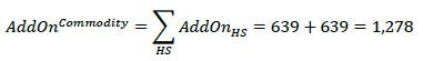 |
| 12.76. | The aggregate netting set level add-on can now be calculated. As set out in 6.27, it is calculated as the sum of the asset class level add-ons. That is for this example:
|
| | 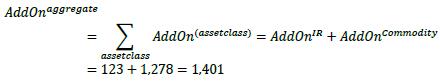 |
| 12.77. | As can be seen from 12.63, the value of V-C is negative (i.e. -120) and so the multiplier will be less than 1. The multiplier is calculated using the formula set out in 6.25, which for this example gives:
|
| |  |
| 12.78. | Finally, aggregating the replacement cost and the PFE component and multiplying the result by the alpha factor of 1.4, the EAD is as follows (USD thousands):
|
EAD = 1.4 * (0 + 0.958 * 1,401) = 1,879
|
